Impact Function Calibration

CLIMADA provides the climada.util.calibrate module for calibrating impact functions based on impact data. This tutorial will guide through the usage of this module by calibrating an impact function for tropical cyclones (TCs).

For further information on the classes available from the module, see its documentation.

Overview

The basic idea of the calibration is to find a set of parameters for an impact function that minimizes the deviation between the calculated impact and some impact data. For setting up a calibration task, users have to supply the following information:

• Hazard and Exposure (as usual, see the tutorial)

• The impact data to calibrate the model to

• An impact function definition depending on the calibrated parameters

• Bounds and constraints of the calibrated parameters (depending on the calibration algorithm)

• A “cost function” defining the single-valued deviation between impact data and calculated impact

• A function for transforming the calculated impact into the same data structure as the impact data

This information defines the calibration task and is inserted into the Input object. Afterwards, the user may insert this object into one of the optimizer classes. Currently, the following classes are available:

• BayesianOptimizer: Uses Bayesian optimization to sample the parameter space.

• ScipyMinimizeOptimizer: Uses the scipy.optimize.minimize function for determining the best parameter set.

The following tutorial walks through the input data preparation and the setup of a BayesianOptimizer instance for calibration. For a brief example, refer to Quickstart. If you want to go through a somewhat realistic calibration task step-by-step, continue with Calibration Data.

import logging
import climada

logging.getLogger("climada").setLevel("WARNING")

Quickstart

This section gives a very quick overview of assembling a calibration task. Here, we calibrate a single impact function for damage reports in Mexico (MEX) from a TC with IbtracsID 2010176N16278.

import pandas as pd

from climada.util import log_level
from climada.util.api_client import Client
from climada.entity import ImpactFuncSet, ImpfTropCyclone
from climada.util.calibrate import (
    Input,
    BayesianOptimizer,
    BayesianOptimizerController,
    OutputEvaluator,
    msle,
)

# Load hazard and exposure from Data API
client = Client()
exposure = client.get_litpop("MEX")
exposure.gdf["impf_TC"] = 1
all_tcs = client.get_hazard(
    "tropical_cyclone",
    properties={"event_type": "observed", "spatial_coverage": "global"},
)
hazard = all_tcs.select(event_names=["2010176N16278"])

# Impact data (columns: region ID, index: hazard event ID)
data = pd.DataFrame(data=[[2.485465e09]], columns=[484], index=list(hazard.event_id))

# Create input
inp = Input(
    hazard=hazard,
    exposure=exposure,
    data=data,
    # Generate impact function from estimated parameters
    impact_func_creator=lambda v_half: ImpactFuncSet(
        [ImpfTropCyclone.from_emanuel_usa(v_half=v_half, impf_id=1)]
    ),
    # Estimated parameter bounds
    bounds={"v_half": (26, 100)},
    # Cost function
    cost_func=msle,
    # Transform impact to pandas Dataframe with same structure as data
    impact_to_dataframe=lambda impact: impact.impact_at_reg(exposure.gdf["region_id"]),
)

# Set up optimizer (with controller)
controller = BayesianOptimizerController.from_input(inp)
opt = BayesianOptimizer(inp)

# Run optimization
with log_level("WARNING", "climada.engine.impact_calc"):
    output = opt.run(controller=controller)

# Analyse results
output.plot_p_space()
out_eval = OutputEvaluator(inp, output)
out_eval.impf_set.plot()

# Optimal value
output.params

{'v_half': 48.30330871103452}

Follow the next sections of the tutorial for a more in-depth explanation.

Calibration Data

CLIMADA ships data from the International Disaster Database EM-DAT, which we will use to calibrate impact functions on. In the first step, we will select TC events that caused damages in the NA1 basin since 2010.

We use EMDAT data from TCs occurring in the NA1 basin since 2010. We calculate the centroids for which we want to compute the windfields by extracting the countries hit by the cyclones and retrieving a LitPop exposure instance from them. We then use the exposure coordinates as centroids coordinates.

import pandas as pd
from climada.util.constants import SYSTEM_DIR

emdat = pd.read_csv(SYSTEM_DIR / "tc_impf_cal_v01_EDR.csv")
emdat_subset = emdat[(emdat["cal_region2"] == "NA1") & (emdat["year"] >= 2010)]
emdat_subset

	country	region_id	cal_region2	year	EM_ID	ibtracsID	emdat_impact	reference_year	emdat_impact_scaled	climada_impact	...	scale	log_ratio	unique_ID	Associated_disaster	Surge	Rain	Flood	Slide	Other	OtherThanSurge
326	MEX	484	NA1	2010	2010-0260	2010176N16278	2.000000e+09	2014	2.485465e+09	2.478270e+09	...	1.0	-0.002899	2010-0260MEX	True	False	False	True	False	False	True
331	ATG	28	NA1	2010	2010-0468	2010236N12341	1.260000e+07	2014	1.394594e+07	1.402875e+07	...	1.0	0.005920	2010-0468ATG	True	False	False	True	False	False	True
334	MEX	484	NA1	2010	2010-0494	2010257N16282	3.900000e+09	2014	4.846656e+09	4.857140e+09	...	1.0	0.002161	2010-0494MEX	True	False	False	True	False	False	True
339	LCA	662	NA1	2010	2010-0571	2010302N09306	5.000000e+05	2014	5.486675e+05	5.492871e+05	...	1.0	0.001129	2010-0571LCA	True	False	False	True	True	False	True
340	VCT	670	NA1	2010	2010-0571	2010302N09306	2.500000e+07	2014	2.670606e+07	2.676927e+07	...	1.0	0.002364	2010-0571VCT	False	False	False	False	False	False	False
344	BHS	44	NA1	2011	2011-0328	2011233N15301	4.000000e+07	2014	4.352258e+07	4.339898e+07	...	1.0	-0.002844	2011-0328BHS	False	False	False	False	False	False	False
345	DOM	214	NA1	2011	2011-0328	2011233N15301	3.000000e+07	2014	3.428317e+07	3.404744e+07	...	1.0	-0.006900	2011-0328DOM	True	False	False	True	False	False	True
346	PRI	630	NA1	2011	2011-0328	2011233N15301	5.000000e+08	2014	5.104338e+08	5.139659e+08	...	1.0	0.006896	2011-0328PRI	True	False	False	True	False	False	True
352	MEX	484	NA1	2011	2011-0385	2011279N10257	2.770000e+07	2014	3.084603e+07	3.077374e+07	...	1.0	-0.002346	2011-0385MEX	True	False	False	True	True	False	True
359	MEX	484	NA1	2012	2012-0276	2012215N12313	3.000000e+08	2014	3.283428e+08	3.284805e+08	...	1.0	0.000419	2012-0276MEX	False	False	False	False	False	False	False
365	MEX	484	NA1	2012	2012-0401	2012166N09269	5.550000e+08	2014	6.074341e+08	6.103254e+08	...	1.0	0.004749	2012-0401MEX	False	False	False	False	False	False	False
369	JAM	388	NA1	2012	2012-0410	2012296N14283	1.654200e+07	2014	1.548398e+07	1.548091e+07	...	1.0	-0.000198	2012-0410JAM	False	False	False	False	False	False	False
406	MEX	484	NA1	2014	2014-0333	2014253N13260	2.500000e+09	2014	2.500000e+09	2.501602e+09	...	1.0	0.000640	2014-0333MEX	True	False	False	True	False	False	True
427	MEX	484	NA1	2015	2015-0470	2015293N13266	8.230000e+08	2014	9.242430e+08	9.239007e+08	...	1.0	-0.000370	2015-0470MEX	True	False	False	True	False	False	True
428	CPV	132	NA1	2015	2015-0473	2015242N12343	1.100000e+06	2014	1.281242e+06	1.282842e+06	...	1.0	0.001248	2015-0473CPV	False	False	False	False	False	False	False
429	BHS	44	NA1	2015	2015-0479	2015270N27291	9.000000e+07	2014	8.362720e+07	1.129343e+06	...	1.0	-4.304733	2015-0479BHS	True	True	False	True	False	False	True
437	MEX	484	NA1	2016	2016-0319	2016248N15255	5.000000e+07	2014	6.098482e+07	6.088808e+07	...	1.0	-0.001588	2016-0319MEX	True	False	False	True	False	False	True
451	MEX	484	NA1	2017	2017-0334	2017219N16279	2.000000e+06	2014	2.284435e+06	2.285643e+06	...	1.0	0.000529	2017-0334MEX	True	False	False	True	True	False	True
456	ATG	28	NA1	2017	2017-0381	2017242N16333	2.500000e+08	2014	2.111764e+08	2.110753e+08	...	1.0	-0.000479	2017-0381ATG	False	False	False	False	False	False	False
457	BHS	44	NA1	2017	2017-0381	2017242N16333	2.000000e+06	2014	1.801876e+06	6.118379e+05	...	1.0	-1.080116	2017-0381BHS	False	False	False	False	False	False	False
458	CUB	192	NA1	2017	2017-0381	2017242N16333	1.320000e+10	2014	1.099275e+10	1.090424e+10	...	1.0	-0.008085	2017-0381CUB	True	False	False	True	False	False	True
459	KNA	659	NA1	2017	2017-0381	2017242N16333	2.000000e+07	2014	1.848489e+07	1.848665e+07	...	1.0	0.000095	2017-0381KNA	False	False	False	False	False	False	False
460	TCA	796	NA1	2017	2017-0381	2017242N16333	5.000000e+08	2014	5.000000e+08	5.003790e+08	...	1.0	0.000758	2017-0381TCA	True	False	False	True	False	False	True
462	VGB	92	NA1	2017	2017-0381	2017242N16333	3.000000e+09	2014	3.000000e+09	6.236200e+08	...	1.0	-1.570826	2017-0381VGB	False	False	False	False	False	False	False
463	DMA	212	NA1	2017	2017-0383	2017260N12310	1.456000e+09	2014	1.534596e+09	8.951186e+08	...	1.0	-0.539066	2017-0383DMA	True	False	False	True	True	False	True
464	DOM	214	NA1	2017	2017-0383	2017260N12310	6.300000e+07	2014	5.481371e+07	5.493466e+07	...	1.0	0.002204	2017-0383DOM	True	False	False	True	True	False	True
465	PRI	630	NA1	2017	2017-0383	2017260N12310	6.800000e+10	2014	6.700905e+10	6.702718e+10	...	1.0	0.000271	2017-0383PRI	True	False	False	True	False	True	True

27 rows × 22 columns

Each entry in the database refers to an economic impact for a specific country and TC event. The TC events are identified by the ID assigned from the International Best Track Archive for Climate Stewardship (IBTrACS). We now want to reshape this data so that impacts are grouped by event and country.

To achieve this, we iterate over the unique track IDs, select all reported damages associated with this ID, and concatenate the results. For missing entries, pandas will set the value to NaN. We assume that missing entries means that no damages are reported (this is a strong assumption), and set all NaN values to zero. Then, we transpose the dataframe so that each row represents an event and each column states the damage for a specific country. Finally, we set the track ID to be the index of the data frame.

track_ids = emdat_subset["ibtracsID"].unique()

data = pd.pivot_table(
    emdat_subset,
    values="emdat_impact_scaled",
    index="ibtracsID",
    columns="region_id",
    # fill_value=0,
)
data

region_id	28	44	92	132	192	212	214	388	484	630	659	662	670	796
ibtracsID
2010176N16278	NaN	NaN	NaN	NaN	NaN	NaN	NaN	NaN	2.485465e+09	NaN	NaN	NaN	NaN	NaN
2010236N12341	1.394594e+07	NaN	NaN	NaN	NaN	NaN	NaN	NaN	NaN	NaN	NaN	NaN	NaN	NaN
2010257N16282	NaN	NaN	NaN	NaN	NaN	NaN	NaN	NaN	4.846656e+09	NaN	NaN	NaN	NaN	NaN
2010302N09306	NaN	NaN	NaN	NaN	NaN	NaN	NaN	NaN	NaN	NaN	NaN	548667.5019	26706058.15	NaN
2011233N15301	NaN	4.352258e+07	NaN	NaN	NaN	NaN	34283168.75	NaN	NaN	5.104338e+08	NaN	NaN	NaN	NaN
2011279N10257	NaN	NaN	NaN	NaN	NaN	NaN	NaN	NaN	3.084603e+07	NaN	NaN	NaN	NaN	NaN
2012166N09269	NaN	NaN	NaN	NaN	NaN	NaN	NaN	NaN	6.074341e+08	NaN	NaN	NaN	NaN	NaN
2012215N12313	NaN	NaN	NaN	NaN	NaN	NaN	NaN	NaN	3.283428e+08	NaN	NaN	NaN	NaN	NaN
2012296N14283	NaN	NaN	NaN	NaN	NaN	NaN	NaN	15483975.86	NaN	NaN	NaN	NaN	NaN	NaN
2014253N13260	NaN	NaN	NaN	NaN	NaN	NaN	NaN	NaN	2.500000e+09	NaN	NaN	NaN	NaN	NaN
2015242N12343	NaN	NaN	NaN	1281242.483	NaN	NaN	NaN	NaN	NaN	NaN	NaN	NaN	NaN	NaN
2015270N27291	NaN	8.362720e+07	NaN	NaN	NaN	NaN	NaN	NaN	NaN	NaN	NaN	NaN	NaN	NaN
2015293N13266	NaN	NaN	NaN	NaN	NaN	NaN	NaN	NaN	9.242430e+08	NaN	NaN	NaN	NaN	NaN
2016248N15255	NaN	NaN	NaN	NaN	NaN	NaN	NaN	NaN	6.098482e+07	NaN	NaN	NaN	NaN	NaN
2017219N16279	NaN	NaN	NaN	NaN	NaN	NaN	NaN	NaN	2.284435e+06	NaN	NaN	NaN	NaN	NaN
2017242N16333	2.111764e+08	1.801876e+06	3.000000e+09	NaN	1.099275e+10	NaN	NaN	NaN	NaN	NaN	18484889.46	NaN	NaN	500000000.0
2017260N12310	NaN	NaN	NaN	NaN	NaN	1.534596e+09	54813712.03	NaN	NaN	6.700905e+10	NaN	NaN	NaN	NaN

This is the data against which we want to compare our model output. Let’s continue setting up the calibration!

Model Setup

In the first step, we create the exposure layer for the model. We use the LitPop module and simply pass the names of all countries listed in our calibration data to the from_countries() classmethod. The countries are the columns in the data object.

Alternatively, we could have inserted emdat_subset["region_id"].unique().tolist().

# from climada.entity.exposures.litpop import LitPop
# from climada.util import log_level

# # Calculate the exposure
# with log_level("ERROR"):
#     exposure = LitPop.from_countries(data.columns.tolist())

from climada.util.api_client import Client
from climada.entity.exposures.litpop import LitPop
from climada.util.coordinates import country_to_iso

client = Client()
exposure = LitPop.concat(
    [
        client.get_litpop(country_to_iso(country_id, representation="alpha3"))
        for country_id in data.columns
    ]
)

from climada.util.api_client import Client

client = Client()
tc_dataset_infos = client.list_dataset_infos(data_type="tropical_cyclone")
client.get_property_values(
    client.list_dataset_infos(data_type="tropical_cyclone"),
    known_property_values={"event_type": "observed", "spatial_coverage": "global"},
)

{'res_arcsec': ['150'],
 'event_type': ['observed'],
 'spatial_coverage': ['global'],
 'climate_scenario': ['None']}

We will use the CLIMADA Data API to download readily computed wind fields from TC tracks. The API provides a large dataset containing all historical TC tracks. We will download them and then select the subset of TCs for which we have impact data by using select().

from climada.util.api_client import Client

client = Client()
all_tcs = client.get_hazard(
    "tropical_cyclone",
    properties={"event_type": "observed", "spatial_coverage": "global"},
)
hazard = all_tcs.select(event_names=track_ids.tolist())

NOTE: Discouraged! This will usually take a longer time than using the Data API

Alternatively, CLIMADA provides the TCTracks class, which lets us download the tracks of TCs using their IBTrACS IDs. We then have to equalize the time steps of the different TC tracks.

The track and intensity of a cyclone are insufficient to compute impacts in CLIMADA. We first have to re-compute a windfield from each track at the locations of interest. For consistency, we simply choose the coordinates of the exposure.

# NOTE: Uncomment this to compute wind fields yourself

# from climada.hazard import Centroids, TCTracks, TropCyclone

# # Get the tracks for associated TCs
# tracks = TCTracks.from_ibtracs_netcdf(storm_id=track_ids.tolist())
# tracks.equal_timestep(time_step_h=1.0, land_params=False)
# tracks.plot()

# # Calculate windfield for the tracks
# centroids = Centroids.from_lat_lon(exposure.gdf['latitude'], exposure.gdf['longitude'])
# hazard = TropCyclone.from_tracks(tracks, centroids)

Calibration Setup

We are now set up to define the specifics of the calibration task. First, let us define the impact function we actually want to calibrate. We select the formula by Emanuel (2011), for which a shortcut exists in the CLIMADA code base: from_emanuel_usa(). The sigmoid-like impact function takes three parameters, the wind threshold for any impact v_thresh, the wind speed where half of the impact occurs v_half, and the maximum impact factor scale. According to the model by Emanuel (2011), v_thresh is considered a constant, so we choose to only calibrate the latter two.

Any CLIMADA Optimizer will roughly perform the following algorithm:

1. Create a set of parameters and built an impact function (set) from it.

2. Compute an impact with that impact function set.

3. Compare the impact and the calibration data via the cost/target function.

4. Repeat N times or until the target function goal is reached.

The selection of parameters is based on the target function varies strongly between different optimization algorithms.

For the first step, we have to supply a function that takes the parameters we try to estimate and returns the impact function set that can later be used in an impact calculation. We only calibrate a single function for the entire basin, so this is straightforward.

To ensure the impact function is applied correctly, we also have to set the impf_ column of the exposure GeoDataFrame. Note that the default impact function ID is 1, and that the hazard type is "TC".

from climada.entity import ImpactFuncSet, ImpfTropCyclone

# Match impact function and exposure
exposure.gdf["impf_TC"] = 1


def impact_func_tc(v_half, scale):
    return ImpactFuncSet([ImpfTropCyclone.from_emanuel_usa(v_half=v_half, scale=scale)])

We will be using the BayesianOptimizer, which requires very little information on the parameter space beforehand. One crucial information are the bounds of the parameters, though. Initial values are not needed because the optimizer first samples the bound parameter space uniformly and then iteratively “narrows down” the search. We choose a v_half between v_thresh and 150, and a scale between 0.01 (it must never be zero) and 1.0. Specifying the bounds as dictionary (a must in case of BayesianOptimizer) also serves the purpose of naming the parameters we want to calibrate. Notice that these names have to match the arguments of the impact function generator.

bounds = {"v_half": (25.8, 150), "scale": (0.01, 1)}

Defining the cost function is crucial for the result of the calibration. You can choose what is best suited for your application. Often, it is not clear which function works best, and it’s a good idea to try out a few. Because the impacts of different events may vary over several orders of magnitude, we select the mean squared logartihmic error (MSLE). This one and other error measures are readily supplied by the sklearn package.

The cost function must be defined as a function that takes the impact object calculated by the optimization algorithm and the input calibration data as arguments, and that returns a single number. This number represents a “cost” of the parameter set used for calculating the impact. A higher cost therefore is worse, a lower cost is better. Any optimizer will try to minimize the cost.

Note that the impact object is an instance of Impact, whereas the input calibration data is a pd.DataFrame. To compute the MSLE, we first have to transform the impact into the same data structure, meaning that we have to aggregate the point-wise impacts by event and country. The function performing this transformation task is provided to the Input via its impact_to_dataframe attribute. Here we choose climada.engine.impact.Impact.impact_at_reg(), which aggregates over countries by default. To improve performance, we can supply this function with our known region IDs instead of re-computing them in every step.

Computations on data frames align columns and indexes. The indexes of the calibration data are the IBTrACS IDs, but the indexes of the result of impact_at_reg are the hazard event IDs, which at this point are only integer numbers. To resolve that, we adjust our calibration dataframe to carry the respective Hazard.event_id as index.

data = data.rename(
    index={
        hazard.event_name[idx]: hazard.event_id[idx]
        for idx in range(len(hazard.event_id))
    }
)
data.index.rename("event_id", inplace=True)
data

region_id	28	44	92	132	192	212	214	388	484	630	659	662	670	796
event_id
1333	NaN	NaN	NaN	NaN	NaN	NaN	NaN	NaN	2.485465e+09	NaN	NaN	NaN	NaN	NaN
1339	1.394594e+07	NaN	NaN	NaN	NaN	NaN	NaN	NaN	NaN	NaN	NaN	NaN	NaN	NaN
1344	NaN	NaN	NaN	NaN	NaN	NaN	NaN	NaN	4.846656e+09	NaN	NaN	NaN	NaN	NaN
1351	NaN	NaN	NaN	NaN	NaN	NaN	NaN	NaN	NaN	NaN	NaN	548667.5019	26706058.15	NaN
1361	NaN	4.352258e+07	NaN	NaN	NaN	NaN	34283168.75	NaN	NaN	5.104338e+08	NaN	NaN	NaN	NaN
3686	NaN	NaN	NaN	NaN	NaN	NaN	NaN	NaN	3.084603e+07	NaN	NaN	NaN	NaN	NaN
3691	NaN	NaN	NaN	NaN	NaN	NaN	NaN	NaN	6.074341e+08	NaN	NaN	NaN	NaN	NaN
1377	NaN	NaN	NaN	NaN	NaN	NaN	NaN	NaN	3.283428e+08	NaN	NaN	NaN	NaN	NaN
1390	NaN	NaN	NaN	NaN	NaN	NaN	NaN	15483975.86	NaN	NaN	NaN	NaN	NaN	NaN
3743	NaN	NaN	NaN	NaN	NaN	NaN	NaN	NaN	2.500000e+09	NaN	NaN	NaN	NaN	NaN
1421	NaN	NaN	NaN	1281242.483	NaN	NaN	NaN	NaN	NaN	NaN	NaN	NaN	NaN	NaN
1426	NaN	8.362720e+07	NaN	NaN	NaN	NaN	NaN	NaN	NaN	NaN	NaN	NaN	NaN	NaN
3777	NaN	NaN	NaN	NaN	NaN	NaN	NaN	NaN	9.242430e+08	NaN	NaN	NaN	NaN	NaN
3795	NaN	NaN	NaN	NaN	NaN	NaN	NaN	NaN	6.098482e+07	NaN	NaN	NaN	NaN	NaN
1450	NaN	NaN	NaN	NaN	NaN	NaN	NaN	NaN	2.284435e+06	NaN	NaN	NaN	NaN	NaN
1454	2.111764e+08	1.801876e+06	3.000000e+09	NaN	1.099275e+10	NaN	NaN	NaN	NaN	NaN	18484889.46	NaN	NaN	500000000.0
1458	NaN	NaN	NaN	NaN	NaN	1.534596e+09	54813712.03	NaN	NaN	6.700905e+10	NaN	NaN	NaN	NaN

Execute the Calibration

We created a class BayesianOptimizerController to control and guide the calibration process. It is intended to walk through several optimization iterations and stop the process if the best guess cannot be improved. The optimization works as follows:

1. The optimizer randomly samples the parameter space init_points times.

2. The optimizer uses a Gaussian regression process to “smartly” sample the parameter space at most n_iter times.

   • The process uses an “Upper Confidence Bound” sampling method whose parameter kappa indicates how close the sampled points are to the buest guess. Higher kappa means more exploration of the parameter space, lower kappa means more exploitation.

   • After each sample, the parameter kappa is reduced by the factor kappa_decay. By default, this parameter is set such that kappa equals kappa_min at the last step. This way, the sampling becomes more exploitative the more steps are taken.

3. The controller tracks the improvements of the buest guess for parameters. If min_improvement_count consecutive improvements are lower than min_improvement, the smart sampling is stopped. In this case, the iterations count is increased and the process repeated from step 1.

4. If an entire iteration did not show any improvement, the optimization is stopped. It is also stopped when the max_iterations count is reached.

Users can control the “density”, and thus the accuracy of the sampling by adjusting the controller parameters. Increasing init_points, n_iter, min_improvement_count, and max_iterations, and decreasing min_improvement generally increases density and accuracy, but leads to longer runtimes.

We suggest using the from_input classmethod for a convenient choice of sampling density based on the parameter space. The two parameters init_points and n_iter are set to \(b^N\), where \(N\) is the number of estimated parameters and \(b\) is the sampling_base parameter, which defaults to 4.

Now we can finally execute our calibration task! We will plug all input parameters in an instance of Input, and then create the optimizer instance with it. The Optimizer.run method returns an Output object, whose params attribute holds the optimal parameters determined by the calibration.

Notice that the BayesianOptimization maximizes a target function. Therefore, higher target values are better than lower ones in this case.

from climada.util.calibrate import (
    Input,
    BayesianOptimizer,
    BayesianOptimizerController,
    msle,
)

from climada.util import log_level

# Define calibration input
with log_level("INFO", name_prefix="climada.util.calibrate"):
    input = Input(
        hazard=hazard,
        exposure=exposure,
        data=data,
        impact_func_creator=impact_func_tc,
        cost_func=msle,
        impact_to_dataframe=lambda imp: imp.impact_at_reg(exposure.gdf["region_id"]),
        bounds=bounds,
    )

    # Create and run the optimizer
    opt = BayesianOptimizer(input)
    controller = BayesianOptimizerController.from_input(input)
    bayes_output = opt.run(controller=controller)
    bayes_output.params  # The optimal parameters

2025-06-23 13:06:39,791 - climada.util.calibrate.bayesian_optimizer - INFO - Optimization iteration: 0
2025-06-23 13:06:42,001 - climada.util.calibrate.bayesian_optimizer - INFO - Optimization iteration: 1
2025-06-23 13:06:44,417 - climada.util.calibrate.bayesian_optimizer - INFO - Optimization iteration: 2
2025-06-23 13:06:46,862 - climada.util.calibrate.bayesian_optimizer - INFO - Optimization iteration: 3
2025-06-23 13:06:49,665 - climada.util.calibrate.bayesian_optimizer - INFO - Optimization iteration: 4
2025-06-23 13:06:52,649 - climada.util.calibrate.bayesian_optimizer - INFO - Optimization iteration: 5
2025-06-23 13:06:55,998 - climada.util.calibrate.bayesian_optimizer - INFO - Optimization iteration: 6
2025-06-23 13:06:59,703 - climada.util.calibrate.bayesian_optimizer - INFO - No improvement. Stop optimization.

Evaluate Output

The Bayesian Optimizer returns the entire paramter space it sampled via BayesianOptimizerOutput We can find out a lot about the relation of the fitted parameters by investigating how the cost function value depends on them. We can retrieve the parameter space as pandas.DataFrame via p_space_to_dataframe(). This dataframe has MultiIndex columns. One group are the Parameters, the other holds information on the Calibration for each parameter set. Notice that the optimal parameter set is not necessarily the last entry in the parameter space!

p_space_df = bayes_output.p_space_to_dataframe()
p_space_df

	Parameters		Calibration
	scale	v_half	Cost Function
Iteration
0	0.422852	115.264302	2.726950
1	0.010113	63.349706	4.133135
2	0.155288	37.268453	0.800611
3	0.194398	68.718642	1.683610
4	0.402800	92.721038	2.046407
...	...	...	...
219	0.711724	51.676718	0.773888
220	0.920147	48.767230	0.771611
221	0.903951	50.001947	0.765957
222	1.000000	52.968157	0.764202
223	0.799533	49.721016	0.765107

224 rows × 3 columns

In contrast, the controller only tracks the consecutive improvements of the best guess.

controller.improvements()

	iteration	random	target	improvement
sample
0	0	True	-2.726950	inf
2	0	True	-0.800611	2.406088
24	0	False	-0.793780	0.008605
29	0	False	-0.791065	0.003432
40	1	False	-0.781115	0.012737
44	1	False	-0.777910	0.004119
48	1	False	-0.774136	0.004876
60	1	False	-0.773844	0.000377
81	2	False	-0.770928	0.003782
87	2	False	-0.770386	0.000704
89	2	False	-0.768256	0.002773
117	3	False	-0.765309	0.003850
123	3	False	-0.765110	0.000260
156	4	False	-0.764939	0.000223
178	5	False	-0.763951	0.001294
189	5	False	-0.763910	0.000054

To get one group of the columns, simply access the item.

p_space_df["Parameters"]

	scale	v_half
Iteration
0	0.422852	115.264302
1	0.010113	63.349706
2	0.155288	37.268453
3	0.194398	68.718642
4	0.402800	92.721038
...	...	...
219	0.711724	51.676718
220	0.920147	48.767230
221	0.903951	50.001947
222	1.000000	52.968157
223	0.799533	49.721016

224 rows × 2 columns

Notice that the optimal parameter set is not necessarily the last entry in the parameter space! Therefore, let’s order the parameter space by the ascending cost function values.

p_space_df = p_space_df.sort_values(("Calibration", "Cost Function"), ascending=True)
p_space_df

	Parameters		Calibration
	scale	v_half	Cost Function
Iteration
189	1.000000	52.392753	0.763910
178	1.000000	52.176364	0.763951
185	1.000000	52.647234	0.763968
222	1.000000	52.968157	0.764202
180	1.000000	51.656629	0.764398
...	...	...	...
139	0.081255	145.935720	5.822272
35	0.028105	118.967924	6.298332
97	0.012842	102.449398	6.635728
204	0.031310	143.537900	7.262185
101	0.025663	141.236104	7.504095

224 rows × 3 columns

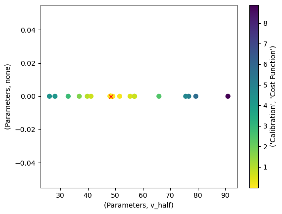
The BayesianOptimizerOutput supplies the plot_p_space() method for convenience. If there were more than two parameters we calibrated, it would produce a plot for each parameter combination.

bayes_output.plot_p_space(x="v_half", y="scale")

<Axes: xlabel='(Parameters, v_half)', ylabel='(Parameters, scale)'>

p_space_df["Parameters"].iloc[0, :].to_dict()

{'scale': 1.0, 'v_half': 52.392753384866985}

Analyze the Calibration

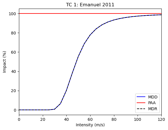
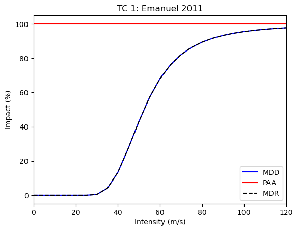
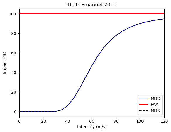
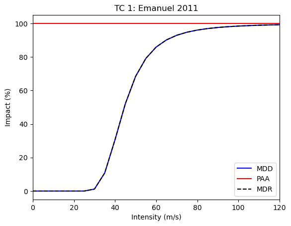
Now that we obtained a calibration result, we should investigate it further. The tasks of evaluating results and plotting them is simplified by the OutputEvaluator. It takes the input and output of a calibration task as parameters. Let’s start by plotting the optimized impact function:

from climada.util.calibrate import OutputEvaluator

output_eval = OutputEvaluator(input, bayes_output)
output_eval.impf_set.plot()

<Axes: title={'center': 'TC 1: Emanuel 2011'}, xlabel='Intensity (m/s)', ylabel='Impact (%)'>

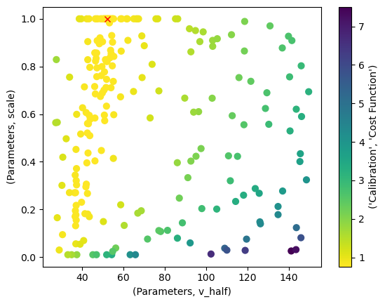
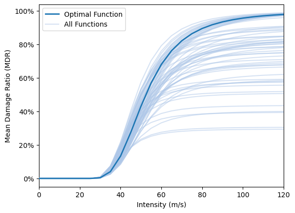
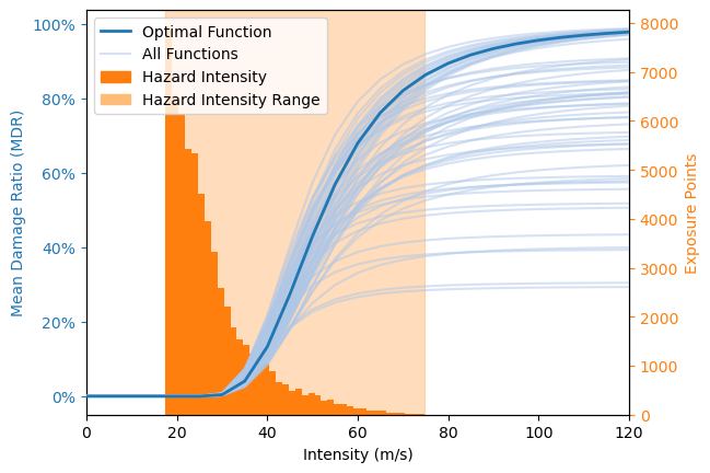
Here we show how the variability in parameter combinations with similar cost function values (as seen in the plot of the parameter space) translate to varying impact functions. In addition, the hazard value distribution is shown. Together this provides an intuitive overview regarding the robustness of the optimization, given the chosen cost function. It does NOT provide a view of the sampling uncertainty (as e.g. bootstrapping or cross-validation) NOR of the suitability of the cost function which is chosen by the user.

This functionality is only available from the BayesianOptimizerOutputEvaluator tailored to Bayesian optimizer outputs. It includes all function from OutputEvaluator.

from climada.util.calibrate import BayesianOptimizerOutputEvaluator, select_best

output_eval = BayesianOptimizerOutputEvaluator(input, bayes_output)

# Plot the impact function variability
output_eval.plot_impf_variability(select_best(p_space_df, 0.03), plot_haz=False)
output_eval.plot_impf_variability(select_best(p_space_df, 0.03))

<Axes: xlabel='Intensity (m/s)', ylabel='Mean Damage Ratio (MDR)'>

The target function has limited meaning outside the calibration task. To investigate the quality of the calibration, it is helpful to compute the impact with the impact function defined by the optimal parameters. The OutputEvaluator readily computed this impact when it was created. You can access the impact via the impact attribute.

import numpy as np

impact_data = output_eval.impact.impact_at_reg(exposure.gdf["region_id"])
impact_data.set_index(np.asarray(hazard.event_name), inplace=True)
impact_data

	28	44	92	132	192	212	214	388	484	630	659	662	670	796
2010176N16278	0.000000e+00	0.000000e+00	0.000000e+00	0.000000	0.000000e+00	0.000000e+00	0.000000e+00	0.000000e+00	1.629343e+09	0.000000e+00	0.000000e+00	0.000000e+00	0.000000e+00	0.000000e+00
2010236N12341	2.362421e+07	0.000000e+00	6.273895e+07	0.000000	0.000000e+00	0.000000e+00	0.000000e+00	0.000000e+00	0.000000e+00	7.489799e+07	1.243066e+07	0.000000e+00	0.000000e+00	0.000000e+00
2010257N16282	0.000000e+00	0.000000e+00	0.000000e+00	0.000000	0.000000e+00	0.000000e+00	0.000000e+00	0.000000e+00	9.210669e+07	0.000000e+00	0.000000e+00	0.000000e+00	0.000000e+00	0.000000e+00
2010302N09306	0.000000e+00	0.000000e+00	0.000000e+00	0.000000	0.000000e+00	0.000000e+00	0.000000e+00	0.000000e+00	0.000000e+00	0.000000e+00	0.000000e+00	6.668112e+06	4.537917e+06	6.931670e+05
2011233N15301	0.000000e+00	1.221974e+09	2.344844e+07	0.000000	0.000000e+00	0.000000e+00	7.044665e+04	0.000000e+00	0.000000e+00	7.033207e+08	0.000000e+00	0.000000e+00	0.000000e+00	1.374375e+08
2011279N10257	0.000000e+00	0.000000e+00	0.000000e+00	0.000000	0.000000e+00	0.000000e+00	0.000000e+00	0.000000e+00	3.687471e+06	0.000000e+00	0.000000e+00	0.000000e+00	0.000000e+00	0.000000e+00
2012215N12313	0.000000e+00	0.000000e+00	0.000000e+00	0.000000	0.000000e+00	0.000000e+00	0.000000e+00	0.000000e+00	1.564085e+08	0.000000e+00	0.000000e+00	0.000000e+00	0.000000e+00	0.000000e+00
2012166N09269	0.000000e+00	0.000000e+00	0.000000e+00	0.000000	0.000000e+00	0.000000e+00	0.000000e+00	0.000000e+00	1.890366e+08	0.000000e+00	0.000000e+00	0.000000e+00	0.000000e+00	0.000000e+00
2012296N14283	0.000000e+00	1.311881e+08	0.000000e+00	0.000000	2.742997e+09	0.000000e+00	0.000000e+00	3.077018e+09	0.000000e+00	0.000000e+00	0.000000e+00	0.000000e+00	0.000000e+00	0.000000e+00
2014253N13260	0.000000e+00	0.000000e+00	0.000000e+00	0.000000	0.000000e+00	0.000000e+00	0.000000e+00	0.000000e+00	1.353240e+10	0.000000e+00	0.000000e+00	0.000000e+00	0.000000e+00	0.000000e+00
2015293N13266	0.000000e+00	0.000000e+00	0.000000e+00	0.000000	0.000000e+00	0.000000e+00	0.000000e+00	0.000000e+00	9.395908e+08	0.000000e+00	0.000000e+00	0.000000e+00	0.000000e+00	0.000000e+00
2015242N12343	0.000000e+00	0.000000e+00	0.000000e+00	225671.780693	0.000000e+00	0.000000e+00	0.000000e+00	0.000000e+00	0.000000e+00	0.000000e+00	0.000000e+00	0.000000e+00	0.000000e+00	0.000000e+00
2015270N27291	0.000000e+00	8.412341e+05	0.000000e+00	0.000000	0.000000e+00	0.000000e+00	0.000000e+00	0.000000e+00	0.000000e+00	0.000000e+00	0.000000e+00	0.000000e+00	0.000000e+00	0.000000e+00
2016248N15255	0.000000e+00	0.000000e+00	0.000000e+00	0.000000	0.000000e+00	0.000000e+00	0.000000e+00	0.000000e+00	3.107738e+09	0.000000e+00	0.000000e+00	0.000000e+00	0.000000e+00	0.000000e+00
2017219N16279	0.000000e+00	0.000000e+00	0.000000e+00	0.000000	0.000000e+00	0.000000e+00	0.000000e+00	0.000000e+00	9.019579e+07	0.000000e+00	0.000000e+00	0.000000e+00	0.000000e+00	0.000000e+00
2017242N16333	3.732403e+08	1.348337e+06	4.696049e+08	0.000000	3.351103e+09	0.000000e+00	2.670109e+07	0.000000e+00	0.000000e+00	1.164926e+10	4.024997e+08	0.000000e+00	0.000000e+00	8.060703e+08
2017260N12310	0.000000e+00	0.000000e+00	3.385997e+07	0.000000	0.000000e+00	6.658893e+08	1.178713e+08	0.000000e+00	0.000000e+00	8.941185e+10	0.000000e+00	0.000000e+00	0.000000e+00	9.182423e+07

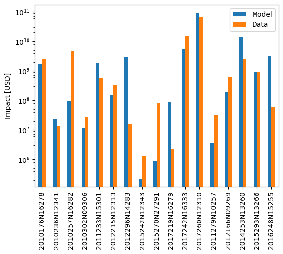
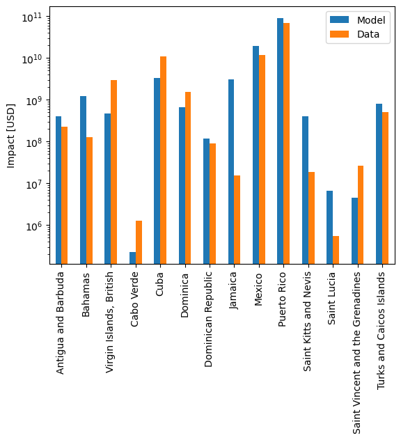
We can now compare the modelled and reported impact data on a country- or event-basis. The OutputEvaluator also has methods for that. In both of these, you can supply a transformation function with the data_transf argument. This transforms the data to be plotted right before plotting. Recall that we set the event IDs as index for the data frames. To better interpret the results, it is useful to transform them into event names again, which are the IBTrACS IDs. Likewise, we use the region IDs for region identification. It might be nicer to transform these into country names before plotting.

import climada.util.coordinates as u_coord


def country_code_to_name(code):
    return u_coord.country_to_iso(code, representation="name")


event_id_to_name = {
    hazard.event_id[idx]: hazard.event_name[idx] for idx in range(len(hazard.event_id))
}

output_eval.plot_at_event(
    data_transf=lambda x: x.rename(index=event_id_to_name), logy=True
)
output_eval.plot_at_region(
    data_transf=lambda x: x.rename(index=country_code_to_name), logy=True
)

<Axes: ylabel='Impact [USD]'>

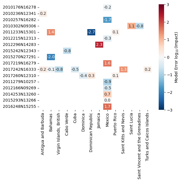
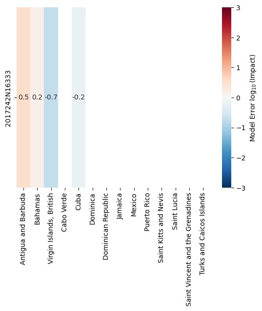
Finally, we can do an event- and country-based comparison using a heatmap using plot_event_region_heatmap() Since the magnitude of the impact values may differ strongly, this method compare them on a logarithmic scale. It divides each modelled impact by the observed impact and takes the the decadic logarithm. The result will tell us how many orders of magnitude our model was off. Again, the considerations for “nicer” index and columns apply.

output_eval.plot_event_region_heatmap(
    data_transf=lambda x: x.rename(index=event_id_to_name, columns=country_code_to_name)
)

<Axes: >

Handling Missing Data

NaN-valued input data has a special meaning in calibration: It implies that the impact calculated by the model for that data point should be ignored. Opposed to that, a value of zero indicates that the model should be calibrated towards an impact of exactly zero for this data point.

There might be instances where data is provided for a certain region or event, and the model produces no impact for them. This is always treated as an impact of zero during the calibration. Likewise, there might be instances where the model computes an impact for a region for which no impact data is available. In these cases, missing_data_value of Input is used as fill value for the data. According to the data value logic mentioned above, missing_data_value=np.nan (the default setting) will cause the modeled impact to be ignored in the calibration. Setting missing_data_value=0, on the other hand, will calibrate the model towards zero impact for all regions or events where no data is supplied.

Let’s exemplify this with a subset of the data used for the last calibration. Irma is the cyclone with ID 2017242N16333, and it hit most locations we were looking at before. It has the event ID 1454 in our setup. Let’s just use this hazard and the related data for now.

NOTE: We must pass a dataframe to the input, but selecting a single row or column will return a Series. We expand it into a dataframe again and make sure the new frame is oriented the correct way.

hazard_irma = all_tcs.select(event_names=["2017242N16333"])
data_irma = data.loc[1454, :].to_frame().T
data_irma

region_id	28	44	92	132	192	212	214	388	484	630	659	662	670	796
1454	211176356.8	1801876.321	3.000000e+09	NaN	1.099275e+10	NaN	NaN	NaN	NaN	NaN	18484889.46	NaN	NaN	500000000.0

Let’s first calibrate the impact function only on this event, including all data we have.

from climada.util.calibrate import (
    Input,
    BayesianOptimizer,
    OutputEvaluator,
    msle,
)
import matplotlib.pyplot as plt


def calibrate(hazard, data, **input_kwargs):
    """Calibrate using custom hazard and data"""
    # Define calibration input
    input = Input(
        hazard=hazard,
        exposure=exposure,
        data=data,
        impact_func_creator=impact_func_tc,
        cost_func=msle,
        impact_to_dataframe=lambda imp: imp.impact_at_reg(exposure.gdf["region_id"]),
        bounds=bounds,
        **input_kwargs,
    )

    # Create and run the optimizer
    with log_level("INFO", name_prefix="climada.util.calibrate"):
        opt = BayesianOptimizer(input)
        controller = BayesianOptimizerController.from_input(input)
        bayes_output = opt.run(controller=controller)

    # Evaluate output
    output_eval = OutputEvaluator(input, bayes_output)
    output_eval.impf_set.plot()

    plt.figure()  # New figure because seaborn.heatmap draws into active axes
    output_eval.plot_event_region_heatmap(
        data_transf=lambda x: x.rename(
            index=event_id_to_name, columns=country_code_to_name
        )
    )

    return bayes_output.params  # The optimal parameters

param_irma = calibrate(hazard_irma, data_irma)

2025-04-25 14:27:18,449 - climada.util.calibrate.bayesian_optimizer - INFO - Optimization iteration: 0
2025-04-25 14:27:20,708 - climada.util.calibrate.bayesian_optimizer - INFO - Optimization iteration: 1
2025-04-25 14:27:23,082 - climada.util.calibrate.bayesian_optimizer - INFO - Optimization iteration: 2
2025-04-25 14:27:25,550 - climada.util.calibrate.bayesian_optimizer - INFO - No improvement. Stop optimization.

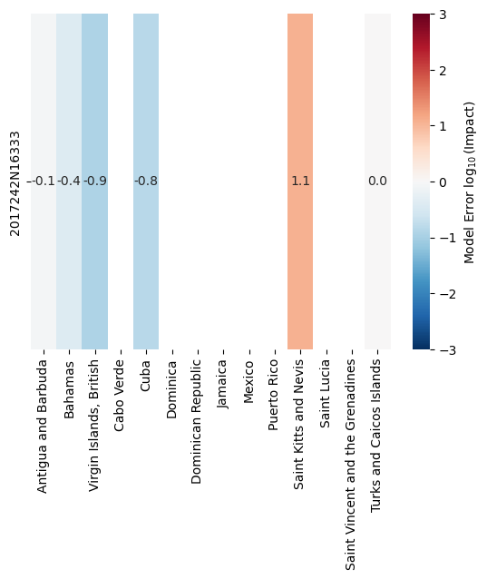
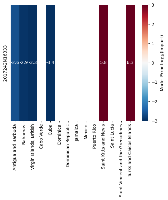
If we now remove some of the damage reports and repeat the calibration, the respective impact computed by the model will be ignored. For Saint Kitts and Nevis, and for Turks and the Caicos Islands, the impact is overestimated by the model. Removing these regions from the estimation should shift the estimated parameters accordingly, because by default, impacts for missing data points are ignored with missing_data_value=np.nan.

calibrate(hazard_irma, data_irma.drop(columns=[659, 796]))

2025-04-25 14:27:38,008 - climada.util.calibrate.bayesian_optimizer - INFO - Optimization iteration: 0
2025-04-25 14:27:40,210 - climada.util.calibrate.bayesian_optimizer - INFO - Optimization iteration: 1
2025-04-25 14:27:42,394 - climada.util.calibrate.bayesian_optimizer - INFO - Optimization iteration: 2
2025-04-25 14:27:44,707 - climada.util.calibrate.bayesian_optimizer - INFO - No improvement. Stop optimization.

{'scale': 1.0, 'v_half': 44.48812601602297}

However, the calibration should change into the other direction once we require the modeled impact at missing data points to be zero:

calibrate(hazard_irma, data_irma.drop(columns=[659, 796]), missing_data_value=0)

2025-04-25 14:27:58,736 - climada.util.calibrate.bayesian_optimizer - INFO - Optimization iteration: 0
2025-04-25 14:28:01,264 - climada.util.calibrate.bayesian_optimizer - INFO - Optimization iteration: 1
2025-04-25 14:28:04,332 - climada.util.calibrate.bayesian_optimizer - INFO - Optimization iteration: 2
2025-04-25 14:28:07,387 - climada.util.calibrate.bayesian_optimizer - INFO - No improvement. Stop optimization.

{'scale': 0.029173288291594105, 'v_half': 110.11137319113446}

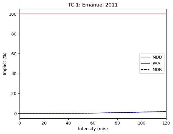
Actively requiring that the model calibrates towards zero impact in the two dropped regions means that it will typically strongly overestimate the impact there (because impact actually took place). This will “flatten” the vulnerability curve, causing strong underestimation in the other regions.

How to Continue

While the found impact function looks reasonable, we find that the model overestimates the impact severely for several events. This might be due to missing data, but it is also strongly related to the choice of impact function (shape) and the particular goal of the calibration task.

The most crucial information in the calibration task is the cost function. The RMSE measure is sensitive to the largest errors (and hence the largest impact). Therefore, using it in the calibration minimizes the overall error, but will incorrectly capture events with impact of lower orders of magnitude. Using a cost function based on the ratio between modelled and observed impact might increase the overall error but decrease the log-error for many events.

So we present some ideas on how to continue and/or improve the calibration:

1. Run the calibration again, but change the number of initial steps and/or iteration steps.

2. Use a different cost function, e.g., an error measure based on a ratio rather than a difference.

3. Also calibrate the v_thresh parameter. This requires adding constraints, because v_thresh < v_half.

4. Calibrate different impact functions for houses in Mexico and Puerto Rico within the same optimization task.

5. Employ the ScipyMinimizeOptimizer instead of the BayesianOptimizer.

Ensemble Calibration

The parameter space of a single calibration task gives an estimate of the uncertainty within that calibration. However, it only gives limited information on the uncertainty stemming from the model setup and impact data provided. To estimate the full model-chain uncertainty, we provide additional method for calibrating ensembles of impact functions based on subsets of the full impact data.

We define two types of ensembles and hence calibration tasks:

• The average ensemble (AE) collects impact functions that are calibrated on sampled subsets of the impact data.

• The ensemble of tragedies (EoT) collects impact functions that are calibrated on a single impact record each.

We provide two classes that calibrate these types of ensembles, namely AverageEnsembleOptimizer and TragedyEnsembleOptimizer. These classes define how the impact data is sampled for each individual impact function calibration task, and then defer this task to an underlying optimizer (which we showcased before). Both take Input object that could also be used in a single calibration optimizer.

Average Ensemble

For each calibration of the AE, we sample the impact data by drawing a fraction of all impact values. In this case, let’s draw the default 80% with an ensemble size of 5, meaning that we compute 5 distinct impact functions. As underlying optimizer, we again choose the BayesianOptimizer. The BayesianOptimizerController is passed via the optimizer_run_kwargs argument of run(). Note that you must provide the type of the underlying optimizer when constructing an EnsembleOptimizer.

from climada.util.calibrate import (
    Input,
    AverageEnsembleOptimizer,
    BayesianOptimizer,
    BayesianOptimizerController,
    msle,
)
from climada.util import log_level

# Define calibration input
with log_level("WARNING", name_prefix="climada.util.calibrate"):
    input = Input(
        hazard=hazard,
        exposure=exposure,
        data=data,
        impact_func_creator=impact_func_tc,
        cost_func=msle,
        impact_to_dataframe=lambda imp: imp.impact_at_reg(exposure.gdf["region_id"]),
        bounds=bounds,
    )

    # Create and run the optimizer
    opt_ae = AverageEnsembleOptimizer(input, optimizer_type=BayesianOptimizer)
    controller = BayesianOptimizerController.from_input(input)
    output_ae = opt_ae.run(controller=controller)

100%|██████████| 20/20 [03:01<00:00,  9.08s/it]

The output of an ensemble optimizer is different from that of a single optimizer. Instead of the parameter space for each optimization we only provide the best estimate of each iteration, along with some information on the events and regions the particular function was calibrated on. We also provide methods for plotting the resulting ensemble of impact functions.

output_ae.data

	Parameters		Event
	scale	v_half	event_id	region_id	event_name
0	0.222773	37.142783	[1333, 1344, 1351, 1361, 3686, 1390, 3743, 142...	[44, 92, 132, 214, 388, 484, 630, 659, 662, 796]	[2010176N16278, 2010257N16282, 2010302N09306, ...
1	1.000000	51.623892	[1333, 1339, 1344, 1351, 1361, 3686, 1377, 374...	[28, 44, 92, 132, 192, 212, 214, 484, 630, 662]	[2010176N16278, 2010236N12341, 2010257N16282, ...
2	1.000000	62.106583	[1339, 1351, 1361, 3686, 3691, 1390, 3743, 142...	[28, 44, 92, 132, 212, 388, 484, 630, 662, 670...	[2010236N12341, 2010302N09306, 2011233N15301, ...
3	1.000000	61.436076	[1339, 1351, 1361, 3691, 1421, 1426, 3777, 379...	[28, 44, 92, 132, 192, 484, 630, 659, 662, 796]	[2010236N12341, 2010302N09306, 2011233N15301, ...
4	0.060143	31.095014	[1333, 1344, 1361, 3686, 3691, 1390, 3743, 379...	[28, 44, 212, 214, 388, 484, 630, 659, 796]	[2010176N16278, 2010257N16282, 2011233N15301, ...
5	1.000000	61.224231	[1333, 1339, 1351, 3691, 1390, 3743, 1421, 377...	[28, 132, 192, 212, 214, 388, 484, 630, 659, 6...	[2010176N16278, 2010236N12341, 2010302N09306, ...
6	0.819839	47.117318	[1333, 1339, 1351, 1361, 3686, 1377, 3743, 142...	[28, 44, 92, 132, 214, 484, 630, 659, 662, 670...	[2010176N16278, 2010236N12341, 2010302N09306, ...
7	1.000000	54.945455	[1333, 1344, 1351, 1361, 3686, 3691, 1377, 139...	[44, 92, 132, 192, 388, 484, 630, 670, 796]	[2010176N16278, 2010257N16282, 2010302N09306, ...
8	0.825518	47.235135	[1339, 1344, 1351, 1361, 3686, 1377, 1390, 374...	[28, 44, 92, 212, 214, 388, 484, 630, 662, 670]	[2010236N12341, 2010257N16282, 2010302N09306, ...
9	1.000000	53.537666	[1339, 1344, 1351, 1361, 3686, 3691, 1390, 374...	[28, 44, 92, 192, 212, 388, 484, 630, 659, 662...	[2010236N12341, 2010257N16282, 2010302N09306, ...
10	1.000000	46.770608	[1344, 1351, 1361, 3691, 1421, 3777, 3795, 145...	[28, 44, 92, 132, 192, 212, 214, 484, 630, 662]	[2010257N16282, 2010302N09306, 2011233N15301, ...
11	0.564386	42.199320	[1344, 1351, 1361, 1377, 1421, 1426, 3777, 145...	[28, 44, 132, 192, 212, 214, 484, 630, 659, 66...	[2010257N16282, 2010302N09306, 2011233N15301, ...
12	1.000000	54.550104	[1333, 1351, 1361, 3686, 3691, 1377, 1426, 379...	[28, 44, 92, 192, 214, 484, 630, 662, 796]	[2010176N16278, 2010302N09306, 2011233N15301, ...
13	0.094194	30.650604	[1333, 1361, 3686, 1377, 1390, 3743, 1421, 379...	[44, 92, 132, 192, 212, 214, 388, 484, 630, 65...	[2010176N16278, 2011233N15301, 2011279N10257, ...
14	0.517233	49.958477	[1333, 1351, 1361, 3691, 1377, 1390, 3743, 377...	[28, 44, 92, 192, 214, 388, 484, 630, 662]	[2010176N16278, 2010302N09306, 2011233N15301, ...
15	0.289714	30.852674	[1339, 1344, 1351, 1361, 3691, 1426, 3777, 379...	[28, 44, 92, 192, 212, 214, 484, 630, 659, 670...	[2010236N12341, 2010257N16282, 2010302N09306, ...
16	0.749633	53.316453	[1333, 1339, 1351, 1361, 3691, 1390, 3743, 142...	[28, 44, 132, 192, 212, 214, 388, 484, 630, 66...	[2010176N16278, 2010236N12341, 2010302N09306, ...
17	1.000000	54.641313	[1333, 1344, 1351, 1361, 3686, 3691, 1377, 374...	[28, 44, 92, 192, 214, 484, 630, 659, 662, 670...	[2010176N16278, 2010257N16282, 2010302N09306, ...
18	0.812884	51.297538	[1333, 1339, 1344, 1351, 1361, 1377, 1390, 374...	[28, 44, 92, 192, 212, 214, 388, 484, 630, 662...	[2010176N16278, 2010236N12341, 2010257N16282, ...
19	1.000000	54.085105	[1333, 1339, 1344, 1351, 1361, 3686, 3691, 137...	[28, 44, 92, 132, 192, 212, 388, 484, 630, 659...	[2010176N16278, 2010236N12341, 2010257N16282, ...

output_ae.plot_shiny(
    impact_func_creator=impact_func_tc,
    haz_type="TC",
    impf_id=1,
    inp=input,
    legend=False,
)

<Axes: title={'center': 'TC 1'}, xlabel='Intensity [m/s]', ylabel='Impact'>

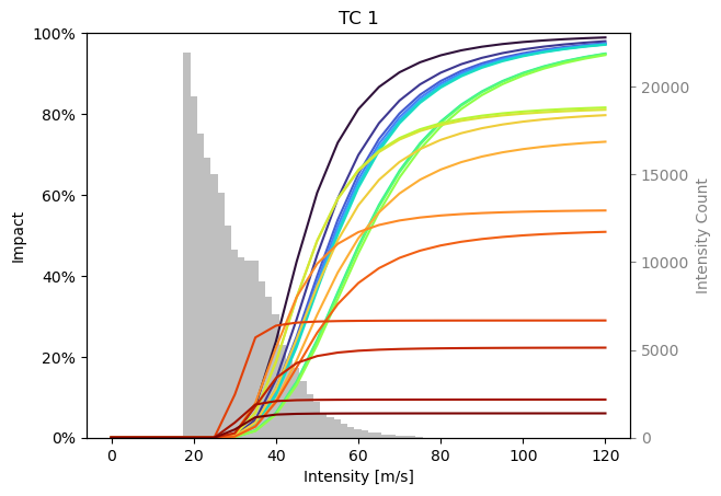
As you can see, although we only resampled the calibration data for each calibration, the functions differ quite a lot. We can investigate exactly which impact records cause this through the ensemble of tragedies. It can be calibrated the same way. By default, it computes one function for every data point in data.

from climada.util.calibrate import TragedyEnsembleOptimizer

# Define calibration input
with log_level("WARNING", name_prefix="climada.util.calibrate"):
    input = Input(
        hazard=hazard,
        exposure=exposure,
        data=data,
        impact_func_creator=impact_func_tc,
        cost_func=msle,
        impact_to_dataframe=lambda imp: imp.impact_at_reg(exposure.gdf["region_id"]),
        bounds=bounds,
    )

    # Create and run the optimizer
    opt_eot = TragedyEnsembleOptimizer(input, optimizer_type=BayesianOptimizer)
    controller = BayesianOptimizerController.from_input(input)
    output_eot = opt_eot.run(controller=controller)

Data point [ 1.  25.8] is not unique. 1 duplicates registered. Continuing ...
Data point [ 1.  25.8] is not unique. 2 duplicates registered. Continuing ...
Data point [ 1.  25.8] is not unique. 3 duplicates registered. Continuing ...

Data point [ 1.  25.8] is not unique. 1 duplicates registered. Continuing ...
Data point [ 1.  25.8] is not unique. 2 duplicates registered. Continuing ...
Data point [ 1.  25.8] is not unique. 3 duplicates registered. Continuing ...

100%|██████████| 27/27 [03:25<00:00,  7.61s/it]

output_eot.data

	Parameters		Event
	scale	v_half	event_id	region_id	event_name
0	0.623918	43.558467	[1333]	[484]	[2010176N16278]
1	0.446720	49.853994	[1339]	[28]	[2010236N12341]
2	0.870346	30.882206	[1344]	[484]	[2010257N16282]
3	0.332453	68.510883	[1351]	[662]	[2010302N09306]
4	0.659666	38.132968	[1351]	[670]	[2010302N09306]
5	0.501478	92.838101	[1361]	[44]	[2011233N15301]
6	1.000000	25.800000	[1361]	[214]	[2011233N15301]
7	0.577457	50.142499	[1361]	[630]	[2011233N15301]
8	0.285608	31.604609	[3686]	[484]	[2011279N10257]
9	0.257775	30.957414	[3691]	[484]	[2012166N09269]
10	0.409814	40.494643	[1377]	[484]	[2012215N12313]
11	0.455964	148.659015	[1390]	[388]	[2012296N14283]
12	0.190400	50.537864	[3743]	[484]	[2014253N13260]
13	0.665652	37.430581	[1421]	[132]	[2015242N12343]
14	1.000000	25.800000	[1426]	[44]	[2015270N27291]
15	0.563058	46.037049	[3777]	[484]	[2015293N13266]
16	0.522021	112.298359	[3795]	[484]	[2016248N15255]
17	1.000000	117.135848	[1450]	[484]	[2017219N16279]
18	0.473914	50.544738	[1454]	[28]	[2017242N16333]
19	0.193221	30.347552	[1454]	[44]	[2017242N16333]
20	1.000000	32.463875	[1454]	[92]	[2017242N16333]
21	0.482094	30.424033	[1454]	[192]	[2017242N16333]
22	0.142128	69.089890	[1454]	[659]	[2017242N16333]
23	1.000000	62.107956	[1454]	[796]	[2017242N16333]
24	1.000000	26.131008	[1458]	[212]	[2017260N12310]
25	0.399726	51.035757	[1458]	[214]	[2017260N12310]
26	0.554834	37.334453	[1458]	[630]	[2017260N12310]

output_eot.plot_shiny(
    impact_func_creator=impact_func_tc,
    haz_type="TC",
    impf_id=1,
    inp=input,
    legend=True,
)

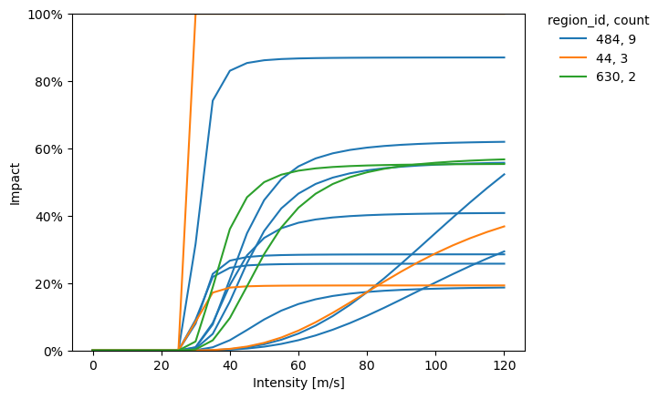
<Axes: title={'center': 'TC 1'}, xlabel='Intensity [m/s]', ylabel='Impact'>

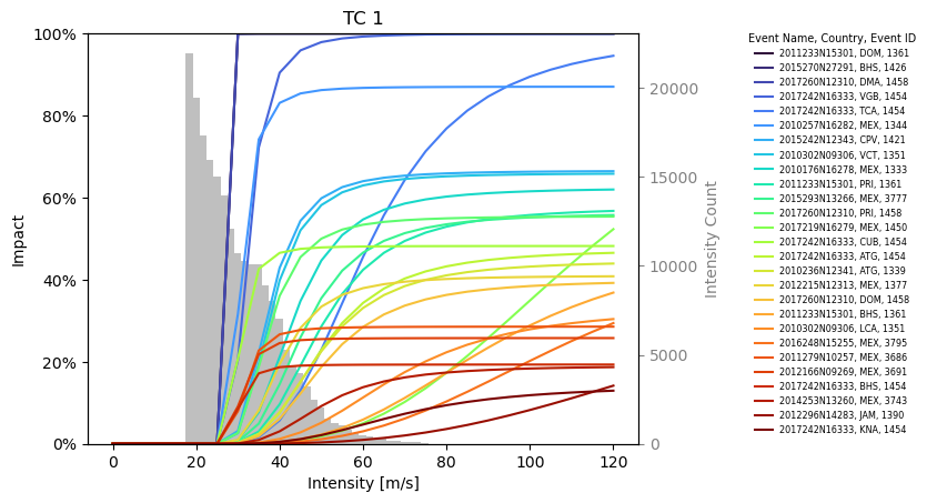
The plot_category function helps to differentiate between impact functions by plotting functions of one category with the same color. Any data in the Event column of the data attribute in the output data may be used.

from climada.util.coordinates import country_to_iso


def to_iso(country):
    return country_to_iso(country, "numeric")


output_eot.plot_category(
    impact_func_creator=impact_func_tc,
    haz_type="TC",
    impf_id=1,
    category="region_id",
    category_colors={to_iso("MEX"): "C0", to_iso("BHS"): "C1", to_iso("PRI"): "C2"},
)

<Axes: xlabel='Intensity [m/s]', ylabel='Impact'>